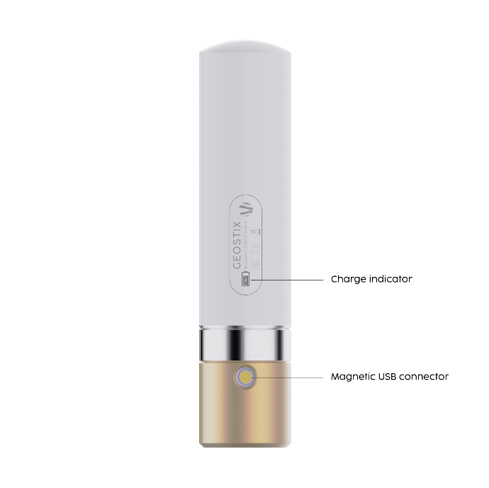
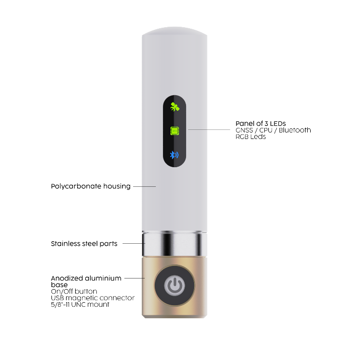
GEOSTIX
High-end GNSS receiver
High accuracy
Achieve a few millimeters of accuracy.
Modularity
Plug additional layers like LTE, 868 MHz RF, solar panel or even your custom sensor layer.
Single form factor
Free to switch between single and multi-frequency GNSS receiver.
Ultra low power
Up to 20 hours of autonomy.

GEOSTIX-M8
SINGLE
FREQUENCY

RECOMMENDED APPLICATIONS

RTK performance
Horizontal accuracy:
2.5 cm + 1 PPM
Vertical accuracy:
5 cm + 1 PPM
LOW COST
ULTRA LOW POWER CONSUMPTION

GEOSTIX-F9
DUAL
FREQUENCY

RECOMMENDED APPLICATIONS


RTK performance
Horizontal accuracy:
1 cm + 1 PPM
Vertical accuracy:
2 cm + 1 PPM
L-BAND CORRECTIONS
LOW POWER CONSUMPTION

GEOSTIX-X5
TRIPLE+
FREQUENCY

RECOMMENDED APPLICATIONS

RTK performance
Horizontal accuracy:
0.6 cm + 0.5 PPM
Vertical accuracy:
1 cm + 1 PPM
L-BAND CORRECTIONS
HIGH-END & HIGHEST RELIABILITY
GNSS RECEIVER
Select the relevant GEOSTIX
In the illustration below, the various accuracy classes are indicated on the left, while the different types of possible applications are listed at the top: post-processing, without an internet link (white zones), local monitoring network or RTK, with an internet connection via 4G/5G.
Boxes M8, F9, K8 and X5 correspond to GEOSTIX-M8, GEOSTIX-F9, GEOSTIX-K8 and GEOSTIX-X5 respectively.

Choose the most appropriate type of correction
Without any correction, GNSS technology achieves accuracy of the order of 5 m in the best conditions.
Fortunately, there are many mechanisms to obtain corrections and considerably improve the accuracy of position measurements.
Except in the case of post-processing, where the data from the GNSS receiver and the corrections converge on the same processing machine, the corrections must reach the GNSS receiver.
These corrections can be transmitted using Ethernet, 3G/4G/5G or directly from one or more satellites.

Corrections are transmitted from one or more known fixed stations to the GNSS receiver operating in rover mode.
It is a differential calculation on the code and not on the phase (RTK), which is why the accuracy does not go below 60 cm.
Corrections are computed from a network of stations observations and then are uploaded to a geostationary satellite.
This satellite, which is dedicated to a specific geographical area, broadcasts corrections via L1 frequency
and is tracked using a channel on the receiver.
Here is a list of the different SBAS in different regions:
- USA: Wide Area Augmentation System (WAAS)
- Europe : European Geostationary Navigation Overlay Service (EGNOS)
- Japan: Michibiki Satellite Augmentation System (MSAS)
- India: GPS-aided GEO-Augmented Navigation (GAGAN)
- China: BeiDou SBAS (BDSBAS) (in development)
- South Korea: Korea Augmentation Satellite System (KASS) (in development)
- Russia: System for Differential Corrections and Monitoring (SDCM) (in development)
- ASECNA: Augmented NaviGation for Africa (ANGA) (in development)
- Australia and New Zealand: Southern Positioning Augmentation Network (SouthPAN) (in development)
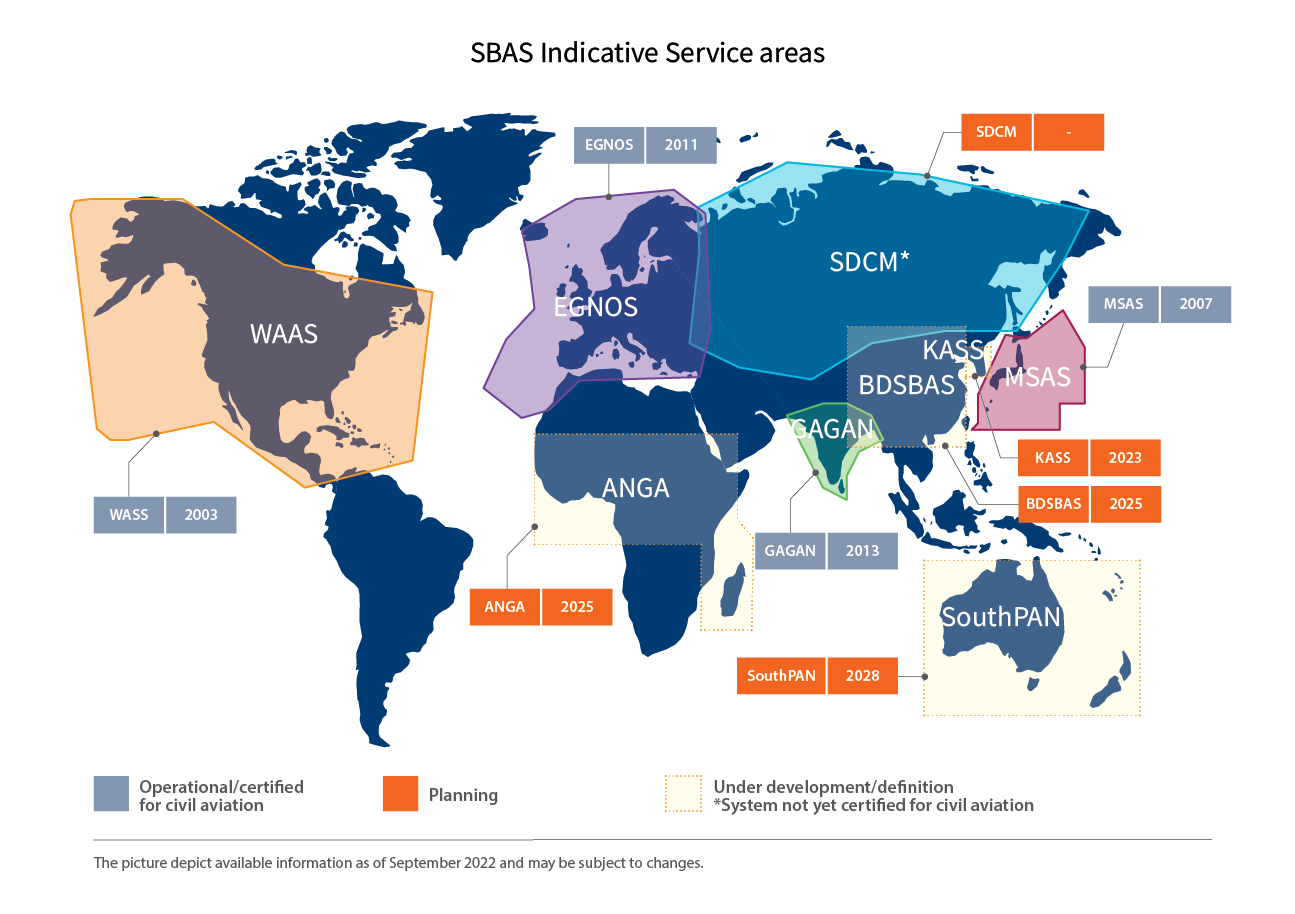
Source: https://www.euspa.europa.eu/european-space/eu-space-programme/what-sbas
Among the many error sources listed in the table below, there are errors originating from the satellites themselves like orbit errors, clock errors and other biases (satellite antenna geometry and phase center).
Thanks to a worldwide network of sparse reference stations that measure orbit or clock imperfections, corrections can be calculated to compensate for these satellite errors.
In PPP operation, GNSS signals are therefore corrected for satellite errors, but other errors remain: atmospheric, multipath and receiver imperfections.
In the case of PPP, there is a fairly high convergence time of around 15-30 minutes to achieve a few centimeters of accuracy. This is the time needed to resolve atmospheric effects in particular, as the delays are different for each of the GNSS frequencies captured by multi-frequency receivers such as GEOSTIX-K8 or GEOSTIX-X5.

In case of PPP, the station is not referenced to a local base station so the measured positions are in a terrestrial reference frame (ITRF).
To obtain the position in any reference frame different from ITRF, user equipment needs to apply the appropriate valid transformation parameters between the latest ITRF and the desired reference frame.
In the case of RTK, a base station transmits corrections to a mobile GNSS receiver within a radius of less than 50 km from the base station.
Accuracy is of the order of 1 cm + 1 PPM.
1 PPM (1 part per million) means 1 cm per million centimeters (distance between the mobile and the base) or 1 cm every 10 km.
Thus, the 1 cm + 1 PPM precision expected for a mobile 10 km away from the base is 2 cm, and 6 cm if the mobile is 50 km away from the base.
Convergence time in RTK mode is of the order of a few seconds.